
Mapware’s Photogrammetry Pipeline, Part 5 of 6: Fusion
In the fusion step of the photogrammetry pipeline, Mapware merges all its depth maps together into a dense 3D point cloud and orients it in real-world space.
Photogrammetry pipeline so far
In the previous pipeline step, Mapware used spatial estimates from its sparse 3D point cloud along with metadata from each raw image to generate depth maps showing the elevation of each image pixel. This vastly increased the density of Mapware’s 3D data.
The purpose of fusion
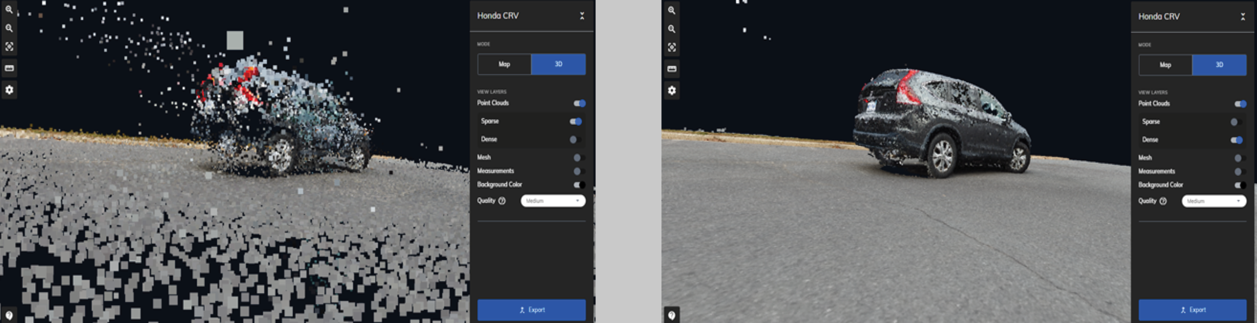
Now, in the fusion step, Mapware takes advantage of its new data to generate a far more-detailed point cloud, filling in the spaces between keypoints. Mapware also georegisters the point cloud (orienting it in real-world latitude/longitude space). The result is far more accurate than anything previously in the pipeline and can serve as the basis of the final 3D digital twin.
Mapware’s fusion process
Dense point cloud generation
First, Mapware brings together the complete list of raw images and depth maps. It also brings together data from all previous pipeline steps including keypoints, image pairings from homography, 3D point estimates from SfM, and pixel elevations from depth mapping.
Then, Mapware runs this data through its stereo fusion algorithms, which project each depth map’s pixels into a temporary 3D space to generate a new point cloud. The code then tries to establish the accuracy of each point by comparing depth maps. If each point is described in at least three depth maps, consensus is reached and the point is considered valid. Otherwise, the point is discarded.
The use of depth map pixels rather than keypoints means that the result is far better than the one generated during the SfM step. Not only are there many more points with fewer gaps between them, but those points are in far more-accurate spatial positions. This is referred to as a high-resolution dense point cloud.
Georegistration
Next, Mapware fits the high-resolution dense 3D point cloud into a real-world coordinates system.
To do this, Mapware reads each raw drone image’s Exchangeable Image File Format (EXIF) metadata to determine the camera’s GPS latitude, longitude, and altitude at the time of each shot. It also retrieves the relative camera positions it calculated earlier during the SfM step. Next, Mapware determines the best linear transformation between those two data sets. With this calculation, along with the relative position of the points in the new dense point cloud, Mapware can determine the position of each point within a real-world coordinates system.
Now that it’s tied to physical coordinates, the dense point cloud can serve as the basis of Mapware’s final 3D digital twin.
Next steps
At this point, Mapware has generated a viable 3D model of the environment. But it is not in a format that many photogrammetry customers want. In the final step of the photogrammetry pipeline, structured output, Mapware will generate additional output formats from its 3D model that users can choose from. We’ll discuss that final step next time.